
Basic Mathematical and Experimental Skills
High School Course Review #1
Pre-Newtonian physics was an entirely alien world of a philosophical and theological concoction.
Its aim ?
To provide a description of the workings of the universe which fit the narrative of a few intellectuals.
But, a paradigm shift occured in the world of physics however, when we stopped asking ‘How?’ and instead began focusing on ‘How much?’.
For the first time in the history of the subject, we were able to provide quantitative descriptions of physical phenomena.
Moreover, by measurement we can compare the efficacy of qualitative explanations based on the accuracy of the predictions made by these quantitative methods.
When I say Basic, I am distinguishing it from its regular connotation of something being Easy.
The word Basic here, refers to the content being the Base of everything that will follow in Physics.
Yet, without these mathematical and experimental skills the conceptual understanding is worthless.
Lessons in this Unit
- Vectors
- Calculus
- Measurements and Error
Vectors
We live in a universe with (atleast) 3 spatial dimensions.
So, the properties of a system (the region of space we are interested in investigating) can vary with space.
When we come across such systems, keeping track of just the magnitude of quantities storing its properties is not enough. We need more information about these quantities. Namely, the direction in which they are acting.
Hence, we employ the greatest thing since sliced bread.
Vectors.
Using vectors, we can store both the magnitude and the direction of the quantity we are interested in. Without this tool, calculations would not only have been cumbersome, but perhaps even impossible.
A Caveat
Note how I slyly jumped to the question of ’what does a vector do ?’, without telling you what it is.
This is because as physics students, we do NOT go too deep into the theory of vectors.
Leave that to the mathematicians !
We are only concerned with vectors (regardless of whatever they may be), because they help us solve problems.
The moment they stop being useful to us (which won’t be the case until we reach classical mechanics), we will throw them in the grabage bin.
Literally.
And this is a recurring theme in physics.
We learn mathematical tools only to the extent of our usage. And pick up the necessary details as we proceed.
Notation
Vectors are represented one of 2 ways.
- A letter with an arrow on top
- A bold letter
This letter may be decided based on convention, for instance F for force.
Or, it may be completely arbitrary.
Sometimes subscripts are added to distinguish more than one quantities of the same kind. For eg. - F1, F2, … Fn
\[F_{1}, F_{2}, ... \;F_{n}\]As mentioned earlier, a vector has both a magnitude, and a direction.
So, we can rewrite a vector as the following :
\[\mathbf{v} = |\vec{v}|\hat{\mathbf{v}} = v\hat{\mathbf{v}}\]Where v (a scalar) is the magnitude and the v^ (v hat) is a unit vector (a vector of magnitude 1) in the direction of v.
Representation
A vector is represented by an arrow of a certain length pointing at a particular direction.
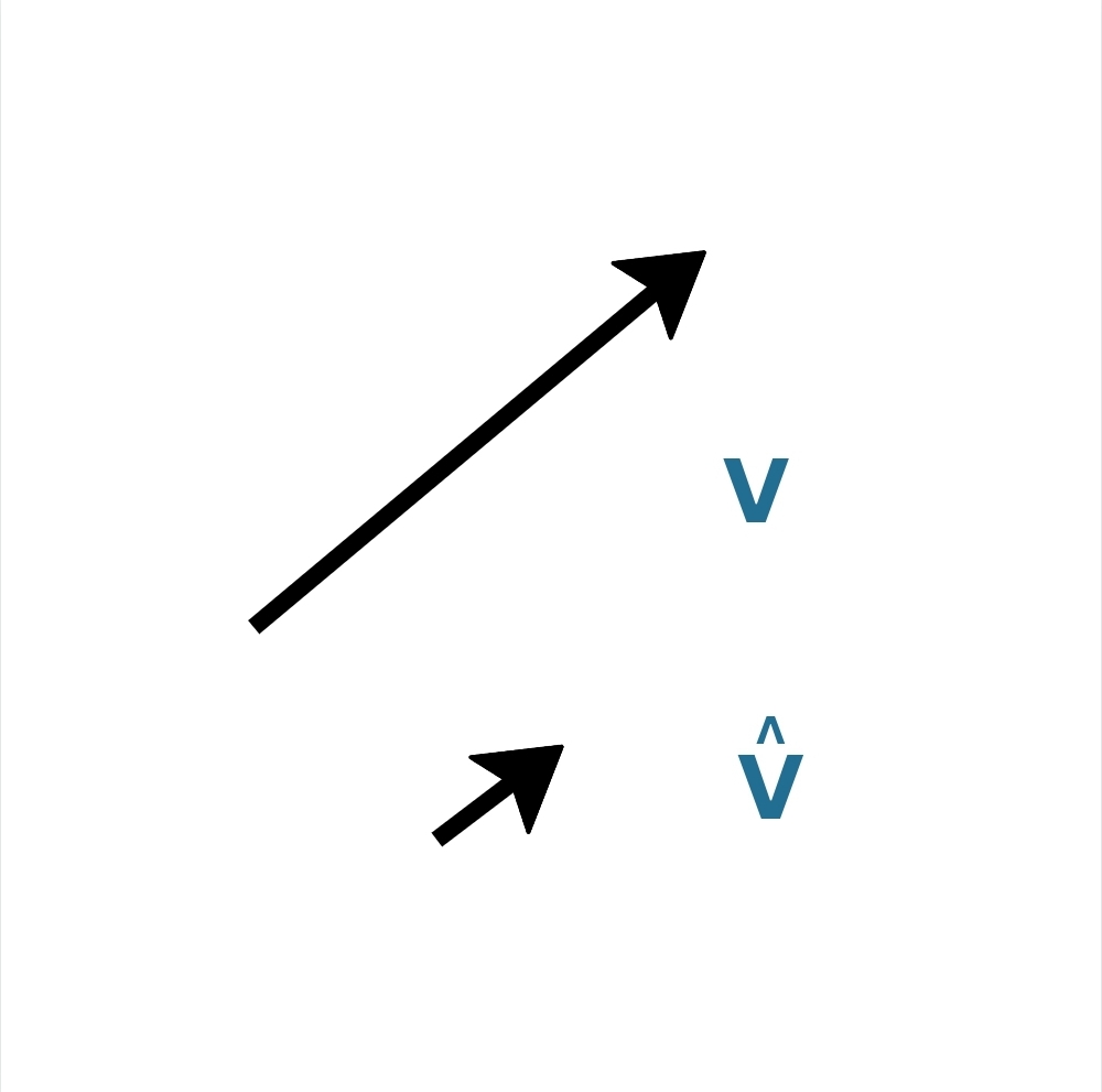
Representation of a vector and its corresponding unit vector
The arrowhead indicates the front of the vector. It comes in handy while adding up vectors.
This also gives us a geometrical interpretation of magnitude (v).
It is simply the number of unit vectors (v^) parallel to the vector you need to add up in order to obtain that vector (v).
Equality of Vectors
If 2 vectors have the same magnitude and are directed in similar directions, they are, by definition equal.
Consequently, if a vector is translated, even then it remains the same.
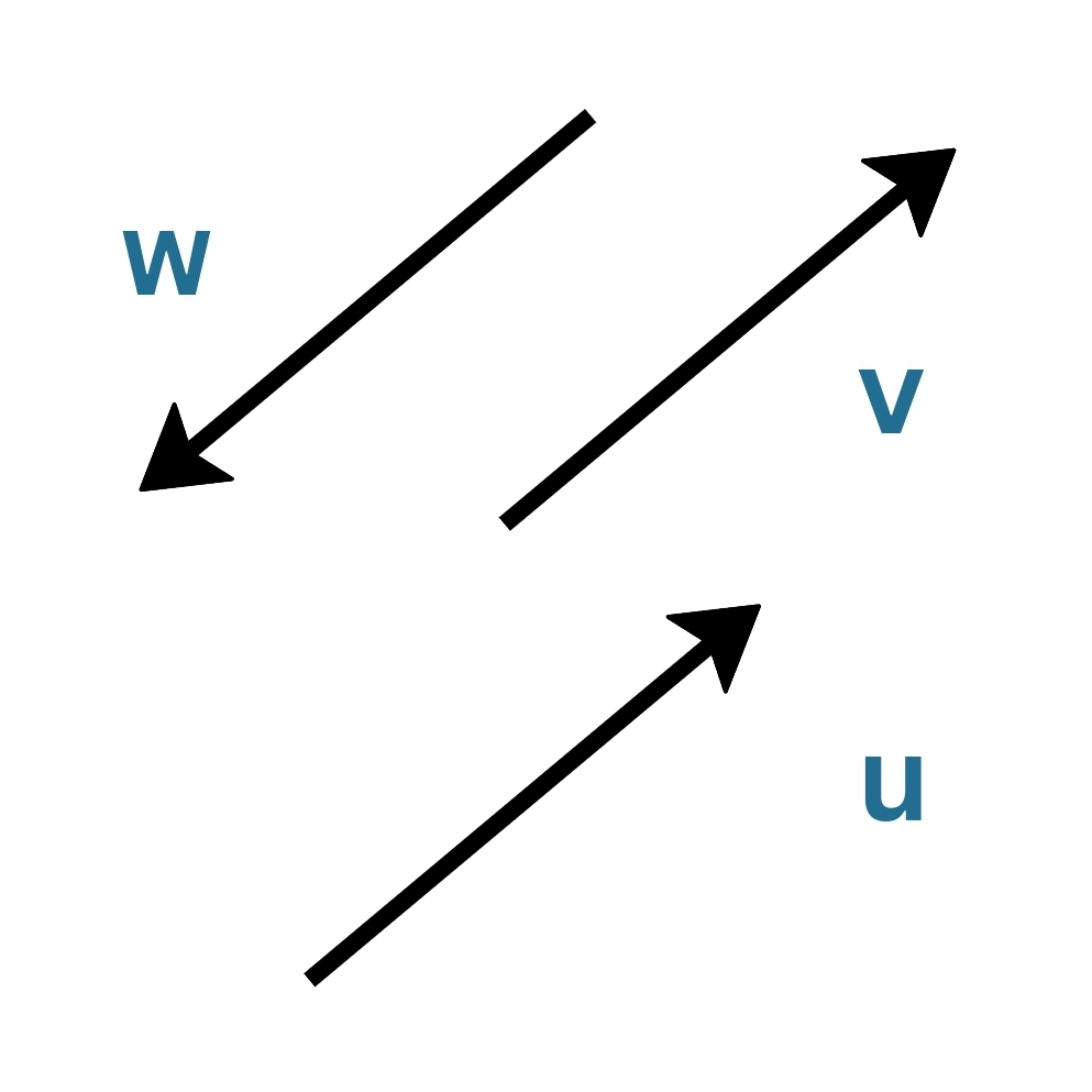
So, in the figure, v = u.
But, v ≠ w.
Even though their magnitudes are same, because the arrowhead is on the other end of, its direction is infact opposite.
As we will come to know, v = - w.
Vector Addition
GIven two vectors u and v, their sum u+v, can be obtained by translating one of them such that its tail lies on the head of the other and joining the tail of the former to the head of the latter.
This can be represented by a triangle or a parallelogram. Hence, the name.
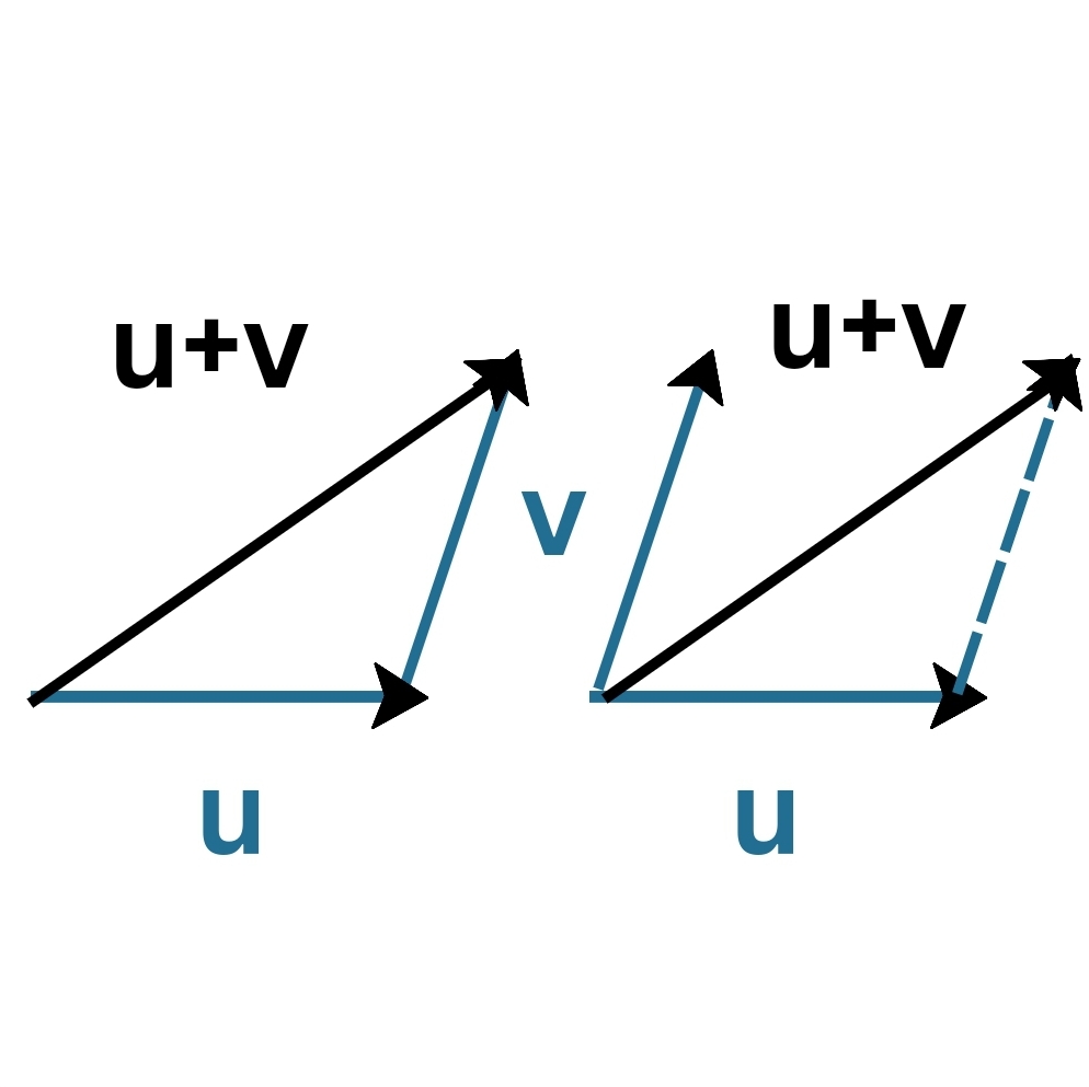
Left : Triangle Law, Right : Parallellgram Law
In case, u and v have the same magnitude, but opposite directions, then u + v = 0.
\[\mathbf{u}+\mathbf{v}=\mathbf{0}\]This vector 0 is called null vector.
It has a magnitude of 0, and has no specified direction.
It is the additive identity for vectors.
That just a fancy way of saying v + 0 = v.
Similarly, - v is called the additive inverse of v, because adding the former to the latter yields the additive identity.
Scalar Multiplication
Multiplication of vector v by a scalar k makes it magnitude kv without changing its direction.
\[k\mathbf{v} = kv\hat{\mathbf{v}}\]i.e. it scales the vector.
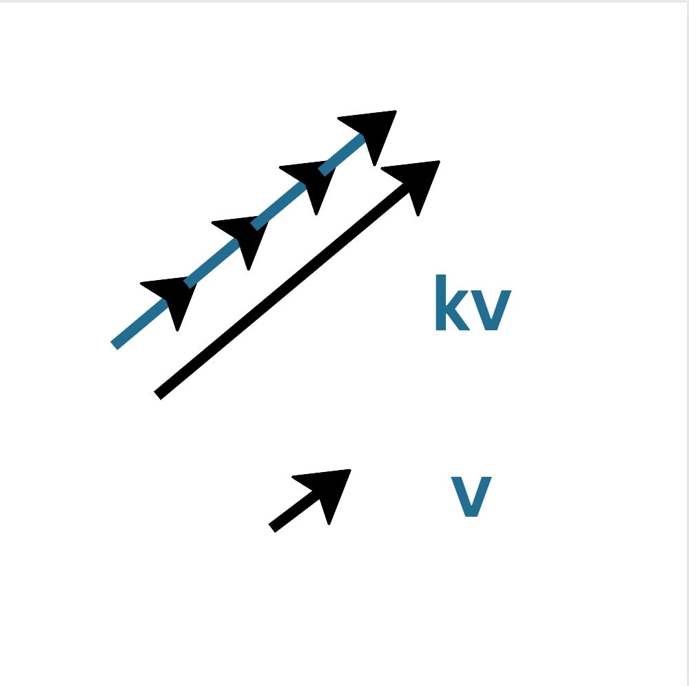
Scalar multiplication of vector is like stacking copies of a vector on top of itself
Coordinate System
When we study a system, we will need to specify the location of objects which are a part of that system.
To do this, we first need a coordinate system.
A coordinate system gives us a way of assigning a set of parameters (coordinates) to each point in space which uniquely determine its position.
The salient feature of a coordinate system is this uniqueness of coordinates assigned to a point.
At the high school level, we will only be dealing with 2D Cartesian Coordinate system.
It looks like this :
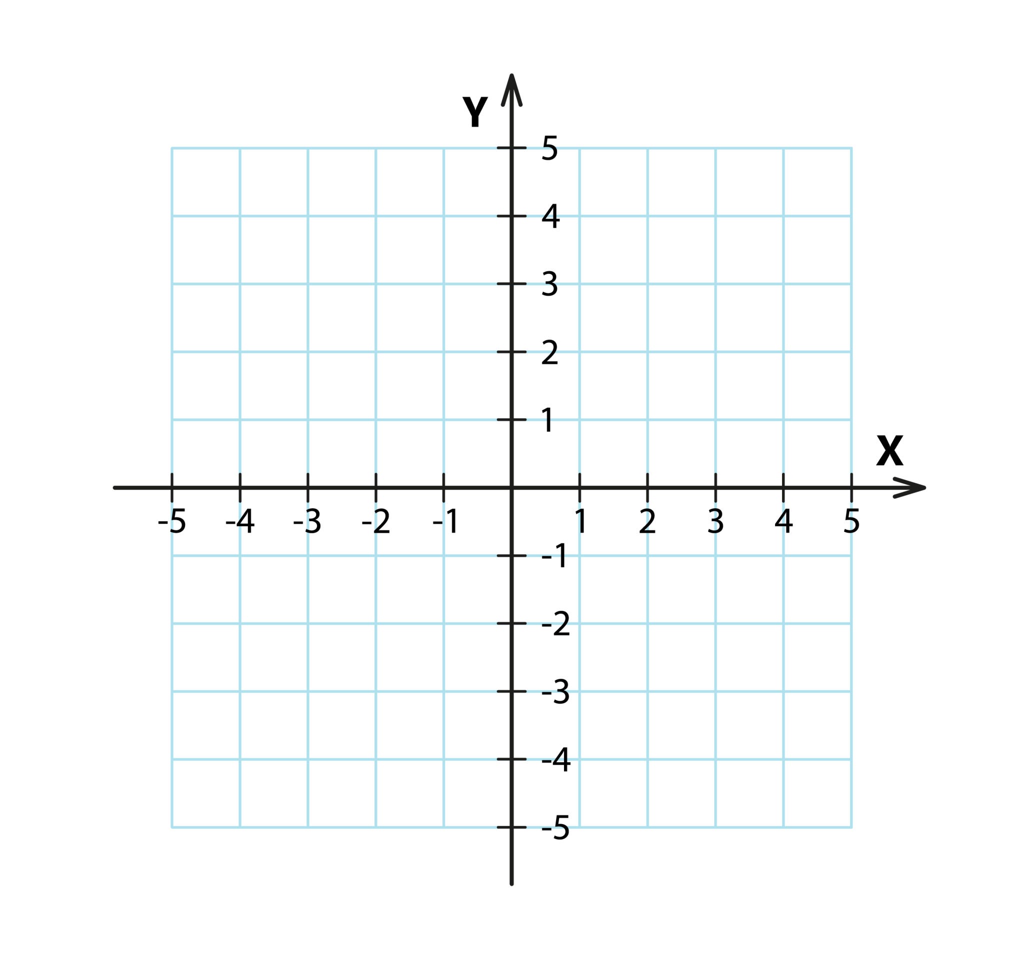
2D Cartesian coordinate system
The axes are labelled as X and Y by convention.
Note that each point is of the form (x,y), where h and k can be any real numbers.
The abcissa (x) represents the distance from the Y axis and the ordinate (y) represents the distance from the X axis.
By convention, the position vector of a point (x,y) is a vector which has its tail at (0,0) and its arrow at the point (x,y).
Since the Cartesian coordinates are defined in terms of relations with the X and Y axes, we would also like any vector to be represented as a sum of vectors along X and Y axes.
To do so, we define unit vectors i^ and j^ along X and Y axes respectively.
Hence, the position vector r of a point (x,y) is the the sum x i^ + y j^.
\[\mathbf{r}= x\hat{\mathbf{i}}+ y\hat{\mathbf{j}}\]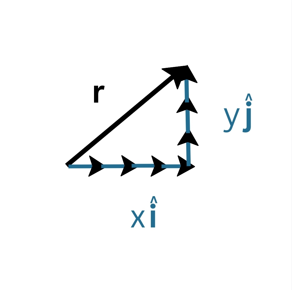
Representing the position vector as a sum of vectors along the X and Y axes
Resolution of Vectors into Components
In the last section, we expressed a given vector as a sum of 2 orthogonal (perpendicular) vectors.
These are called the components of a vector (along and perpendicular to another vector).
Specifically, we calculated the X and Y components of the vector r. But, we are not restricted to taking components along the axes.
In the general, given vectors v and u, we can resolve v into 2 orthogonal vectors - parallel to u and perpendicular to u.
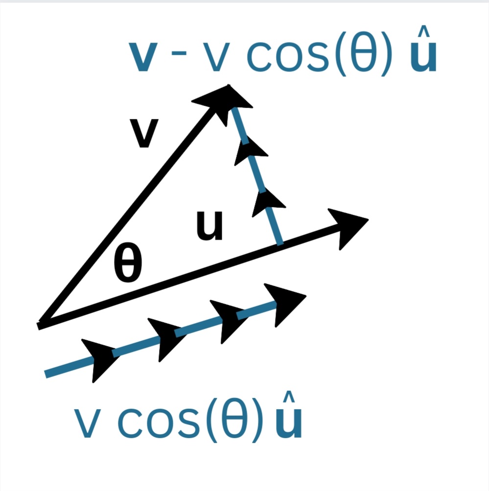
Components of v along and perpendicular to u
If u = i^, we get v = v cos(θ) i^ + v sin(θ) j^
\[\mathbf{v} = v\;cos(\theta)\hat{\mathbf{i}}+v\;sin(\theta)\hat{\mathbf{j}}\]Dot Product (Scalar Product) of 2 vectors
Dot product of 2 vectors u and v is defined as u • v = uv cos(θ).
The operation results in a scalar and is hence also called the scalar product.
It is both commutative and distributive :
- Commutativity
- Distributive
If the vectors
\[\mathbf{u} = u_{x}\hat{\mathbf{i}}+u_{y}\hat{\mathbf{j}}+u_{z}\hat{\mathbf{k}} \\ \mathbf{v} = v_{x}\hat{\mathbf{i}}+v_{y}\hat{\mathbf{j}}+v_{z}\hat{\mathbf{k}}\]Then, their dot product is given by
\[\mathbf{u}\cdot\mathbf{v} = (u_{x}\hat{\mathbf{i}}+u_{y}\hat{\mathbf{j}}+u_{z}\hat{\mathbf{k}})\cdot(v_{x}\hat{\mathbf{i}}+v_{y}\hat{\mathbf{j}}+v_{z}\hat{\mathbf{k}})\] \[= (u_{x}v_{x}\;\hat{\mathbf{i}}\cdot\hat{\mathbf{i}} + u_{y}v_{y}\;\hat{\mathbf{j}}\cdot\hat{\mathbf{j}}+ u_{z}v_{z}\;\hat{\mathbf{k}}\cdot\hat{\mathbf{k}})+2(u_{x}v_{y}\;\hat{\mathbf{i}}\cdot\hat{\mathbf{j}}+u_{y}v_{z}\;\hat{\mathbf{j}}\cdot\hat{\mathbf{k}}+u_{z}v_{x}\;\hat{\mathbf{k}}\cdot\hat{\mathbf{i}})\]Since the axes are perpendicular, the vectors along them are too.
So, θ = 90⁰, making the dot product zero.
\[\hat{\mathbf{i}}\cdot\hat{\mathbf{j}}=\hat{\mathbf{j}}\cdot\hat{\mathbf{k}}= \hat{\mathbf{k}}\cdot\hat{\mathbf{j}}= 0\]Similarly, since the angle between a vector and itself is 0⁰, v•v = vv cos(0⁰) = v^2.
So, for unit vectors,
\[\hat{\mathbf{i}}\cdot\hat{\mathbf{i}}=\hat{\mathbf{j}}\cdot\hat{\mathbf{j}}= \hat{\mathbf{k}}\cdot\hat{\mathbf{k}}= 1\]This makes the dot product of u and v
\[\hat{\mathbf{u}}\cdot\hat{\mathbf{v}}= u_{x}v_{x}+u_{y}v_{y}+u_{z}v_{z}\]Cool.
But why do we care about this dot product all of a sudden ?
Firstly, it lets us calculate those components we were talking about in the last section.
That is, the component of v on u is given by v•u^.
Secondly, this product gives us information about the angle between the 2 vectors (θ).
Rewriting the formula, we obtain a convenient expression for it :
\[cos(\theta) = \frac{\mathbf{u}\cdot\mathbf{v}}{uv}\]Cross Product (Vector Product) of 2 Products
Dot product of 2 vectors u and v is defined as u × v = uv sin(θ) n^.
Where n^ is a vector perpendicular to u^ & v^ and 0≤θ≤π.
If u^ and v^ are non-collinear (i.e. θ≠0⁰), there are exactly 2 vectors which are eligible for being n^.
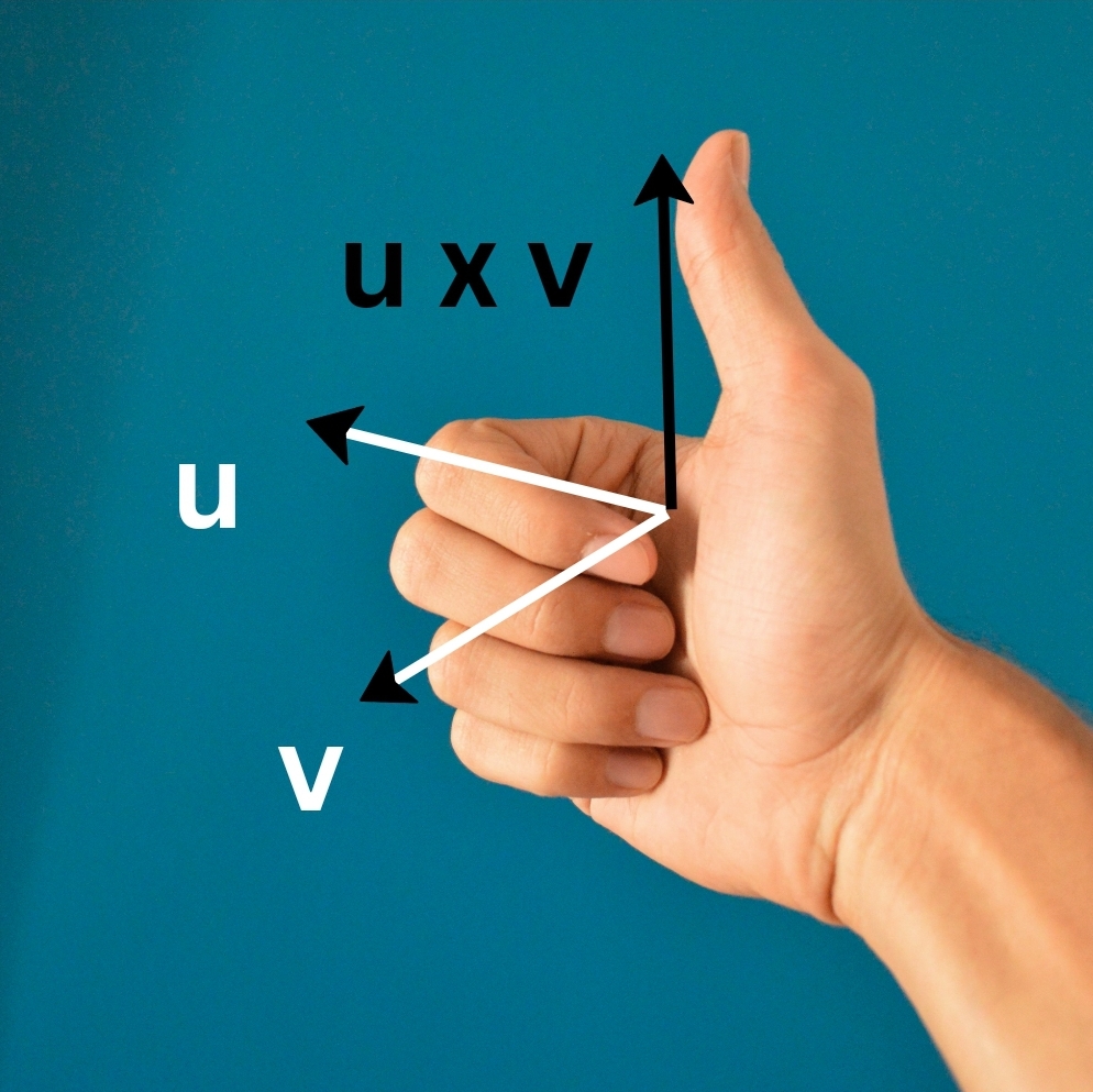
The one chosen is, by convention, determined by the right hand thumb rule.

Direction of u × v for a given u and v is given by the right hand thumb rule
Flatten your palm, all fingers pointing along u. Then curl them towards v such that the angle swept out by the fingers is less that 180⁰.
The thumb points towards the direction of their cross product.
Cross product is non-commutative, i.e.
\[\mathbf{u}×\mathbf{v} \neq \mathbf{v}×\mathbf{u}\]Infact,
\[\mathbf{u}×\mathbf{v} = - \;\mathbf{v}×\mathbf{u}\]But, it does follow distributive law
\[\mathbf{u}×(\mathbf{v}+\mathbf{w})=\mathbf{u}×\mathbf{v}+\mathbf{u}×\mathbf{w}\]In general, cross product helps us work with vectors which a non-planar with u and v.
That is, they cannot be expressed as au + bv, for any real numbers a and b.
Specifically, when we reach Mechanics II, the new quantities we encounter such as torque and angular momentum are defined in terms of cross-products.
Usage
Vectors are especially useful in dealing with multi-dimensional systems in kinematics (check out Mechanics I Course Review for definition) such as a 2-D projectile.
They let us separate the concerns of dealing with both the dimensions at once and instead focus on them separately.
This independence of dimensions lets us simplify the problem from a 2-D projectile (which is novel to us) to two 1-D linear motions (for which we will have already found solutions).
Topics
- Scalars and Vectors
- Vector Notation and Equality
- Vector Operations
- Addition and Subtraction
- Scalar Multiplication
- Resolution of Vectors
- Vector Multiplication
- Scalar (Dot) Product
- Vector (Cross) Product
Experiments
- Measurement of the weight of a given body (a wooden block) using the parallelogram law of vector addition
Calculus
Having solved the problem of describing directions, we now run into another problem.
Vectors sorted our problem of keeping track of space. But, if we wish to describe the phenomenon around us, we need to track its change with time. Changes w.r.t. to time are not always uniform and hence describing rate of change is not an easy job.
Whenever physicists encounter such a situation where they feel they don’t have the right tools to tackle a problem, they delegate the work to fellow mathematicians.
And the humble mathematicians always find a way to help their dear friends.
In this case, we will use a mathematical tool whose contribution to physics is beyond description. Calculus is the mathematical study of continuous changes. And it is precisely this feature of calculus which makes it of so much use to us.
Calculus comes in 2 complementary flavours, namely differential and integral calculus.
Differentiation
Differentiation helps us to calculate the rates of change of quantities with other quantities such as time or position.
This solves our problem of tracking changes.
But first we need to learn about Slope and Limits.
Slope and Limits
In physics, any quantity we are interested in measuring is usually a function of time.
‘Function’ basically means that the value of the quantity changes as the time changes.
We can graph a quantity (let’s say s) which varies with t by plotting them on Y and X axes respectively.
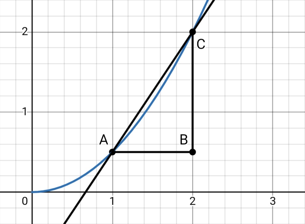
Slope of the graph is given by the ‘rise over run’.
\[\frac{\Delta s}{\Delta t}= \frac{BC}{AB}\]where Δs is a discrete change in the quantity s corresponding to a discrete change Δt in t.
The higher this ratio (slope), the faster s changes with t. This gives us some insight into how s changes with t.
But, notice one thing.
From the graph, it is evident that s changes slower with t around A than it does C.
So, slope only gives us some intermediate or average value between rate of change of s with t at A and at C.
To gain exact information about the rate of change of s with t at A, we would like C to be as close to A as possible.
The as C approaches A, i.e. the closer Δt is to 0, the closer to the ‘real’ or instantaneous rate of change this slope will be.
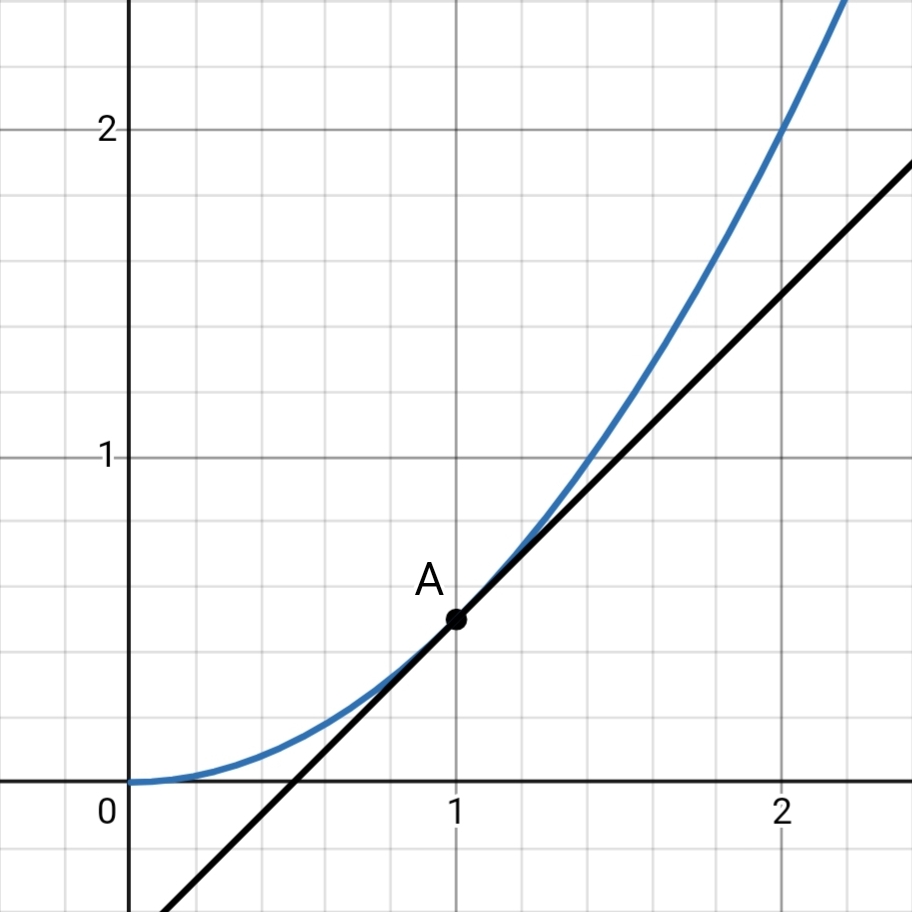
This notion of ‘approaching’ is made rigorous in mathematics using the concept of a limit.
But, for us, limit is nothing more than a tool which helps us magically turn ‘average’ quantities into ‘instantaneous’ ones.
When we apply the limit Δt → 0 the chord AC becomes a tangent to the curve at A. And the slope becomes what is known as a derivative of that function at A.
And just to implicitly state that the limit has been taken, we alter the notation. So, Δs become ds and Δt become dt.
\[\frac{ds}{dt} = \lim_{\Delta t \rightarrow 0} \frac{\Delta s}{\Delta t}\]For our convenience, we may even define this derivative to be a different quantity altogether.
For instance, if we take s to be the displacement (which as we will come to know is actually the symbol used to represent it), its time derivative i.e. derivative w.r.t time is called the velocity.
Integration
With derivatives, we can calculate the instantaneous rates of change.
But in certain situations, we need to calculate quantities based on their given rates of changes. Sometimes, we are also provided with boundary conditions which the quantity must satisfy.
Integration helps us ‘integrate’ this information, in a mathematical sense.
Continuing with the quantity s, let us consider a different scenario.
Suppose we are given rate of change of s with time (say v) and we are required to calculate change in s over a given time interval (say a to b).
Rearranging the expression for average v , we get
\[v_{avg}= \frac{\Delta s}{\Delta t} \\ \Rightarrow \Delta s = v_{avg}\; \Delta t\]We saw that the derivative represented the slope of tangent in ‘s vs t’ graph.
Let’s see what ‘v Δt’ looks like in a ‘v vs t’ graph.
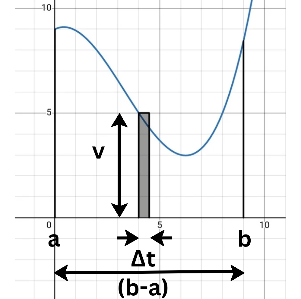
Geometrical significance of v Δt in v vs t graph.
Similar to s, v is also a function of time. So we write that value of v at a time t as v(t).
If v is not uniform (constant), we assume it to be uniform over a small interval of time (Δt). Then, the expression ‘v Δt’ gives us the area of a small sliver of width Δt and height v.
Sum of areas of these slivers, gives us the approximate change in s.
As with the derivative, taking limit of this sum gives us the accurate value.
But, if we take the limit of the sum, geometrically it approaches the area under this ‘v vs t’ graph.
For a certain Δt, there will be N = (b-a)/Δt such slivers.
The net change in s is given by the sum of these Δs.
\[s_{b} - s_{a} = \lim_{\Delta t \rightarrow 0} \Delta s_{0} + \Delta s_{1}+ \ldots + \Delta s_{N} \\ = \lim_{\Delta t \rightarrow 0} v(a)\;\Delta t + v(a+ \Delta t)\;\Delta t + v(a+ 2\Delta t)\;\Delta t + \ldots + v(a+ N\Delta t)\;\Delta t\]To write sums in condensed notation, we use the Greek symbol capital sigma (Σ) and write it as following.
Each value of the iteration variable k gives a term of this sum.
\[s_{b}- s_{a} =\lim_{\Delta t \rightarrow 0} \sum_{k=0}^{N} \Delta s_{k} =\lim_{\Delta t \rightarrow 0} \sum_{k=0}^{N} v(a + k\left(\frac{b-a}{N}\right)) \Delta t\]Now, just as taking limit of the slope gave us a derivative, taking limit of this sum gives us an antiderivative.
It is written as follows
\[s_{b} - s_{a} = \int_{a}^{b} \;ds = \int_{a}^{b} v(t) \;dt\]The antiderivative is
\[\int v(t) \;dt\]The upper and lower bounds (b and a) are the values of t at which this antiderivative has been calculated.
We say, the small change in s (ds = v dt) over this time interval dt has been integrated to find the change in s from a to b.
To calculate s as a function of time, we just select the lower and upper bounds of this antiderivative to be 0 and t instead.
Then we can conveniently substitute the value of intial s (s0) to find the answer.
I have described the process as qualitatively as possible.
Further understanding can only be acquired by rigorous practice of these concepts and their application in problems.
Topics
- Differential Calculus
- Maxima and Minima
- Integral Calculus
Measurements and Errors
‘Any measurement, without the knowledge of its uncertainty is completely meaningless’ - Walter Lewin
Once we have made our hypotheses and relevant mathematical models to describe systems, the next step is to test our predictions. This involves measuring quantities which we derive from experiments.
But, unlike analytic methods, experiments are not perfect.
Hence, our best shot is getting utterly precise. Here, the art of error handling becomes useful.
Errors can seep in from various sources such as faulty equipment, parallax or mishandling of apparatus. To deal with these errors, we must first understand the limits of our measuring devices.
Least Count
Least count of an instrument is the smallest measurement that it can make. Any measurement is only as good as the least count of the instrument used to measure it.
For instance, the least count of the standard 15 cm ruler is 0.1 cm or 1 mm.
But, instead of the humble ruler, we will use the following 2 instruments for taking length measurements at the high school level -
- Vernier Callipers
- Screw Gauge
Vernier Callipers
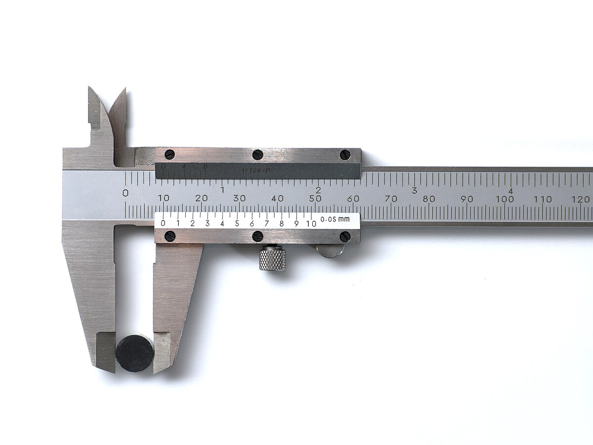
Vernier callipers clamping on an object
(Source : https://en.m.wikipedia.org/wiki/Calipers)
The instrument consists of 2 scales :
- Main scale
- Vernier scale
Main scale is exactly like a regular ruler.
But, in addition, it haa a vernier scale which slides with the teeth of the instrument.
It has smaller markings which can be used to measure lengths smaller than 1 mm.
Here’s how it works -
The difference between the value of one main scale division (MSD) and the value of one vernier scale division (VSD) is known as the least count of the vernier.
It is also known as the vernier constant (VC).
\[VC = 1 \;MSD - 1 \;VSD\]Vernier calipers is designed such that the length of (n − 1) MSD is equal to n VSD.
(for a particular n which is determined by the desired least count for the instrument being designed).
\[(n-1) \;MSD = n \;VSD\]So, the VC becomes
\[VC = 1 \;MSD - 1 \;VSD \\ = 1 \;MSD - \frac{n-1}{n} \; MSD \\ = \frac{1}{n} \;MSD\]For n = 10 and MSD = 1 mm, the least count becomes 0.1 mm.
To measure the outer dimensions of an object, the object is placed in the outer legs. The legs are pushed together until the object is held firmly in place.
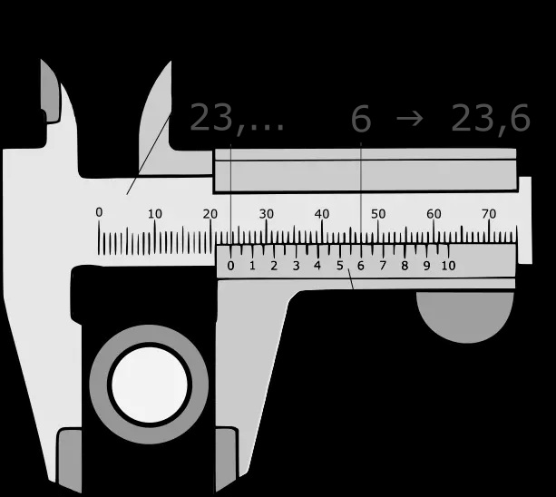
(Source : https://www.aci24.com/en/help-center/faq-help-center/how-do-i-read-a-manual-vernier-caliper.html)
The first significant digit is read from the main scale, immediately to the left of the ‘zero’ on the vernier scale.
In the example shown, this is 23.
The decimal place is now determined on the vernier scale.
The numerical value on the vernier scale is searched for whose scale line lies exactly on top of any scale line on the main scale.
In the example, this is the value 6 on the vernier scale.
This results in a measured value of 23.6 mm.
Screw Gauge
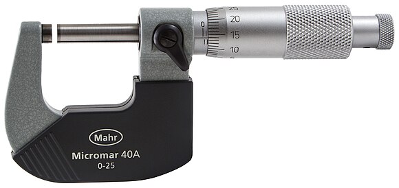
(Source : https://en.m.wikipedia.org/wiki/Micrometer_(device))
It also consists of 2 scales -
- Main scale
- Circular scale
Similar to the vernier calliper, the screw gauge has the same Main scale.
But, instead of having a sliding scale, it has a rotating one operated by a ratchet.
There are 100 markings on the circular scale. A full rotation of the circular scale reveals a portion of the main scale equal to its pitch, which is usually 1 mm (1 MSD).
Therefore 100 circular scale divisons (CSD) are equal to 1 MSD.
\[100 \;CSD = 1 \;MSD \\ 1 \;CSD = \frac{1}{100} \;MSD\]This CSD (0.01 mm), is also the least count of the screw gauge.
To measure the outer dimensions of an object, the object is placed between the anvil and the spindle and held firmly in place.
The main scale reading in the given example is 10.3 mm.
The circular scale reading is the marking on the circular scale coinciding with the line of the main scale.
In this example, it is 43.
So, the total reading is 10.3 mm + 45 CSD = 10.345 mm.
Zero Error
More often than not the ‘zero’ on the vernier or the circular scale does not coincide with that of the main scale.
This may happen due to mishandling of equipment or may even be a result of poor manufacturing.
The value shown by the instrument, where is should have otherwise shown a zero is termed as the zero error.
When the instrument shows a positive reading, it is called positive zero error. In case of the screw gauge, zero error may also be negative, due to the 0 of circular scale being slightly above the main scale line.
To make our readings error-free, we proceed as usual and take the measurements.
Once thet are done, we undo the errors, i.e. we subtract the positive zero error or add the negative zero error to the faulty reading.
This gives us the reading, we should have obtained from an ideal instrument.
Significant Figures
Related to least count is the concept of significant figures.
In any measurement, all the digits present may not be accurate. So, we need to decide which specific digits within a number are necessay in conveying that measurement.
These digits are called significant figure or digits.
Significant figures tell us the reliability of our measurement.
There are certain rules for deciding which digits are significant and which aren’t (details not discussed here).
Any digit in the measurement which is not significant is uncertain and can thus be erroneous. So, there are rules for performing operations (+/-/×/÷) on measurements based of the number of significant digits in them.
Thus, calculations must be done carefully so that the errors do not add up and adultrate the results.
Topics
- Significant Digits
- Calculations using significant digits
- Errors in measurements
Experiments
- Use of Vernier Callipers to
- measure diameter of a small spherical/cylindrical body
- measure the dimensions of a given regular body of known mass and hence to determine its density
- measure the internal diameter and depth of a given cylindrical object like beaker/glass/calorimeter and hence to calculate its volume
- Use of Screw Gauge to
- measure diameter of a given wire
- measure thickness of a given sheet
- determine volume of an irregular lamina
- To determine the radius of curvature of a given spherical surface by a spherometer
Conclusion
Upon the completion of these lessons, you have completed the first step and are already on your way to become a physicist.
You now understand the tools which physicists use daily and are aware of their importance.
Next up, we will learn the foundations of Newtonian mechanics.