Cover Image

When Maxwell wasn’t classy enough

Phasors Revisited

Ok. I have to admit that Maxwell solved a lot of problems in physics.

A lot.

But, was it classy enough ?

Meh.

A problem requires more than just a solution. It requires a solution that is generalizable.

Generalizability comes from application on a wider range of problems of similar kind.

The easier it is to use the solution of a problem as a template for solutions to others, the more generalizable it is.

And thus, all the more classy.

This tale is that of phasors - a classy solution to the circuital analysis of AC circuits.

We will begin with Maxwell’s solution to a problem. And after discussing the historical development of phasors, come back to see if using phasors made any difference.

Physics Without Phasors : Grove’s Series LCR Circuit

In March 1868, a young Maxwell visited William Grove’s laboratory.

In this meeting, he presented Maxwell with a phenomenon he had discovered while working with a induction coil, feeded by an alternating current (AC). Now we know it as resonance in a series LR (inductor-resistor) circuit with an additional capacitor (C) in series, which could be included or excluded from the circuit by the means of a switch.

This configuration is commonly referred to as the series LCR circuit.

Resonance in this AC circuit is characterised by the amplitude of current wave being maximum.

The next morning after the meeting with Grove laboratory, Maxwell addressed him a letter. In the letter, Maxwell calculated the alternating current that passed through the circuit during resonance.

Grove sent this letter to the Philosophical Magazine and it was published in May 1869.

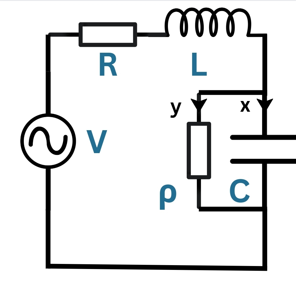
Maxwell’s Circuital Analysis

In the figure, x is the current that circulates in through inductor (inductance L) and resistor (resistance R).

Circuit Diagram for the circuit analysed by Maxwell

For convenience of calculation, he modeled the switch by attaching a resistor in parallel with the capacitor. The value of resistance of this resistor simulates the position of the switch - 0Ω for closed and infinite (∞Ω) for open.

So, let y be the current that passes through the resistor (resistance ρ) in parallel with the capacitor (capacitance C).

The voltage drop in the resistor of resistance ρ is P = ρy.

\[P = \rho y\]

Thus, the charge in the capacitor is

\[C \frac{dP}{dt} = x-y\]

Applying Kirchoff’s Voltage Laws, x obeys the equation

\[Vcos(\omega t)+ Rx+ L\frac{dx}{dt}+ P = 0\]

where V cos ωt is the voltage at the terminals of the AC source.

The key point of the argument is the ansatz - the supposition Maxwell makes to proceed.

He presumed the current x to be of the form

\[x = I\;cos(\omega t+\alpha)\]

Solving for A and from the given equations, he concluded

\[I^2 = \frac{V^2(1+C^2\rho^2\omega^2)}{\rho^2[(1-LC\omega^2)^2+R^2C^2\omega^2]+ 2R\rho+ R^2+ L\omega^2}\]

and

\[\alpha = cot^{-1}\left(\frac{1}{C\rho\omega}\right)- cot^{-1}\left(\frac{R+ \rho- LC\rho\omega^2}{RC\rho\omega+L\omega}\right)\]

For ρ = 0, the switch is closed and a series LR circuit is obtained with

\[I^2 = \frac{V^2}{R^2+ L\omega^2}\]

Alternatively, for ρ = ∞, the switch is open and a series LCR circuit is obtained with

\[I^2 = \frac{V^2}{R^2+ \left(L\omega -\frac{1}{C\omega}\right)^2}\]

The characteristic frequency having ω= 1/sqrt(LC) results in the amplitude of AC current in the circuit being maximum.

\[\omega = \frac{1}{\sqrt{LC}}\]

Thus, this resonant frequency gives the resonance phenomenon in the series LCR circuit with I = V/R

\[I= \frac{V}{R}\]

Maxwell’s analysis is commemdable.

Yet, evidently, he had to force his way through a lot of strenuous calculation.

And all this for a mere series LCR circuit !

AC circuits of exceeding complexity certainly required a novel method for solving.

Challenges posed by AC and the Need for Phasors

Understanding AC current was an enormous challenge back in the end of 19th century.

This is what the electrical engineering legend Charles Steinmetz had to say about the situation :

‘There are two kinds of electric currents in industrial use : Direct currents and alternating currents. The direct current continuously flows in the same direction andits action calculated numerically in a simple manner. The alternating current is a current which continuously changes: It rises from nothing to a maximum,then decreasing again to nothing, reverses direction and decreases again in zero, again reverses and starts againin the first direction, and so on, reversing usually 120 times in a second. Both types of current were used since the early days of electrical engineering, and there was no difficult in making calculations with the direct current: it had a direction and a value, which could be measured by an ammeter.’

Steinmetz also stated that :

‘But the alternating current had no value and no direction; its value continuously changed, and so the direction, and in all calculations with alternating current, instead of a simple mechanical value of the direct current theory, the investigator had to use a complicated function of time to represent the alternating current,and the theory of alternating current apparatus thereby became so complicated that the investigator never got very far. In the meantime the practical electrician who built and ran alternating current machinery, put an ammeter in the alternating current circuit and found that some ammeters (those having permanent magnets) showed nothing, but other ammeters showed a value, and that they called the value of the alternating current. It is what we now call the “effective” or rms value ofthe alternating current. The practical engineering so got a numerical value of the alternating current, but you could not make any calculation with it. For instance, two such alternating currents combined gave a resultant current, which usually was smaller than the sum of the currents and sometimes even smaller than either of the currents.’

The description by Steinmetz makes the crisis absolutely clear. And in such a crisis, the field is desperate for a visionary who steps us and revolutionizes it.

So, Steinmetz took the charge and gave us exactly what we needed.

Steinmetz’s Symbolic Method

In his book, Steinmtez associates a characteristic circle to all sinusoid of the form

\[i(t) = I\;sin(\omega t - \theta)\]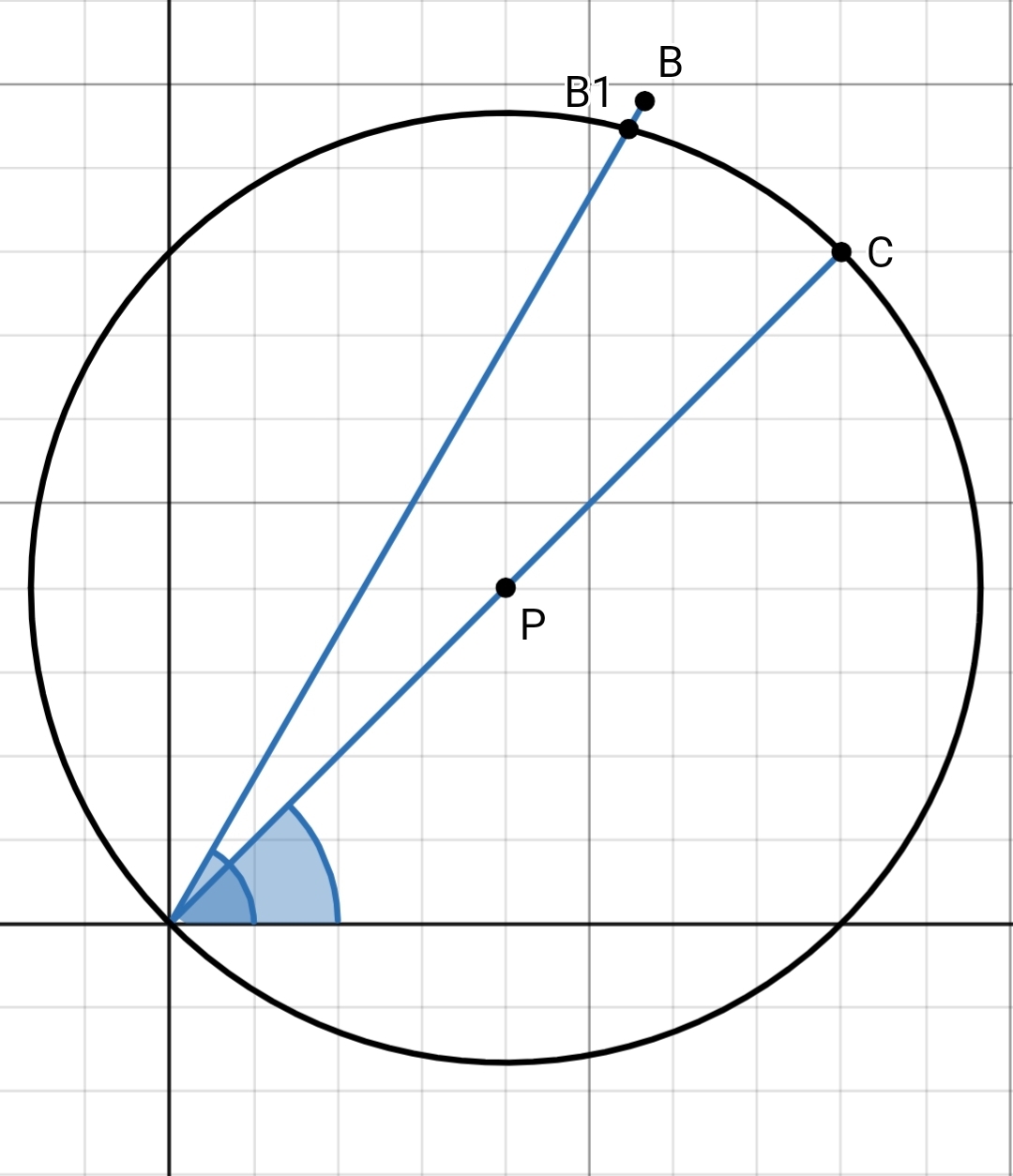

The characteristic circle corresponding to the sinusoid I cos(ωt-θ)

The amplitude I in the sinusoid corresponds to the length of the diameter OC of the characteristic circle.

The angle made by this diameter with the positive x-axis is θ

The figure also shows a line segment OB, whose length is equal to OC and instersects the circle at the point B1.

Angles made by OB and OB1 with the positive x-axis is ωt.

Steinmetz claimed that the instantaneous values of i(t) could be obtained from this OB that rotated with angular velocity ω, by observing the intersection of this line with the characteristic circle.

To do so, Steinmetz had to prove that the length of the chord OB1 was exactly equal to OCcos(ωt-θ).

Proof

Join PB1.

Since OP = OB1 = R (Radius), ΔOPB1 is isosceles.

Therefore, angle B1OP = angle OB1P = (ωt-θ).

Also, since

\[OB_{1} = OP\;cos(\angle B_{1}OP) + B_{1}P\;cos(\angle OB_{1}P)\]

Using the results derived before,

\[OB_{1} = 2R\;cos(\omega t- \theta) \\ =OC\;cos(\omega t- \theta)\]

Since, OC is the diameter of the circle.

Hence, Steinmetz was right.

We could actually encode all the information of a sinusoid in this geometrical construction.

Algebra of Sinusoids and its similarity to Vectors

A sinusoidal wave i(t) = I cos(ωt − θ) can be written as

\[i(t) = I\;cos(\omega t - \theta) \\ = I\;cos(\omega t)\;cos(\theta)+ I\;sin(\omega t)\;sin(\theta)\]

Let us now consider 2 sinusoidal waves i1 and i2 with amplitudes I1 and I2.

\[i_{1}(t) = I_{1}\;cos(\omega t)\;cos(\theta_{1})+ I_{1}\;sin(\omega t)\;sin(\theta_{1}) \\ i_{2}(t) = I_{2}\;cos(\omega t)\;cos(\theta_{2})+ I_{2}\;sin(\omega t)\;sin(\theta_{2})\]

Their sum, i1 + i2 can be calculated as follows.

\[i_{1}(t)+ i_{2}(t)= I_{1}(sin(\omega t)\;cos(\theta_{1})+ cos(\omega t)\;sin(\theta_{1}))+ I_{2}(sin(\omega t)\;cos(\theta_{2})+cos(\omega t)\;sin(\theta_{2}))\] \[= cos(\omega t)(I_{1}\;cos(\theta_{1})+I_{2}\;cos(\theta_{2}))+ sin(\omega t)(I_{1}\;sin(\theta_{1})+I_{2}\;sin(\theta_{2})) \\ = I\;cos(\omega t-\theta)\]

Here’s the interesting part.

Observe that the factor that multiplies cos(ωt) in the expression above is the sum of the horizontal projections of the two diameters of the characteristic circles of the original sinusoids. Similarly, the factor that multiplies the term sin(ωt) is the sum of the vertical projections of the two diameters of the same characteristic circles.

So, the diameter of the sinusoid obtained from the sum of 2 given sinusoids can be represented as a vectorial sum of the two diameters of the individual sinusoids.

Hence, we can essentially work with AC currents by using vectors representing the phase of sinusoidal current.

Infact, the word ‘phasor’ is actually a portmanteau of the term ‘phase vector’.

Tying Phasors to Complex Numbers instead of Vectors

But, we can still do better.

Look, vectors are great.

Yet, whenever rotations are concerned (as in the case of Steinmetz’s geometric representation of the sinusoid), we prefer to use complex numbers.

Because, describing rotations using vectors requires us to use a rotation matrix as a transformation on a given vector. Whereas, to do so using complex numbers requires simply multiplying by a suitable complex number.

So, Steinmetz introduced the concept of complex numbers in circuits analysis.

After proving that the sum of sinusoids could be accomplished through the addition of vectors, he formalized that sine waves are combined, or resolved by adding or subtracting, their rectangular components.

To add complex numbers into the mix, Steinmetz remarked :

“To distinguish the horizontal and vertical components of sine waves, we may mark, for instance, the vertical component with a distinguishing index, as the letter j, and thus represent the sine wave by the expression : i= a + jb

\[i = a+ jb\]

which now has a meaning, that a is the horizontal and b thevertical component of the sine wave i, and that both components are to be combined in a resultant wave of intensity I =a^2 + b^2 and phase θ = arctan(b/a).”

\[I = a^2 + b^2 \\ \theta = arctan\left(\frac{b}{a}\right)\]

He observed that the sinusoid a + jb is perpendicular to the sinusoid −b + ja and claims that this can only occur if j = sqrt(−1).

\[j = \sqrt{-1}\]

Steinmetz said that multiplication by j must also correspond to a rotation of 90⁰ as well.

Deriving the Resonance condition for series LCR using Phasors instead

Even after all the discussion on the historical development, a question still remains.

Did phasors make solution to our original problem of finding the resonance condition and current of series LCR circuit any easier ?

Let’s find out.

Consider a series LCR circuit with an AC Voltage source of voltage amplitude V.

Since the elements are connected in series, the current (I) through them is in phase.

For the resistor, the voltage across it (VR) is in phase with I as well. But, from our previous knowledge of inductor and capacitor, we know that for them, Voltage and Current differ in phase by precisely 90⁰.

Voltage across the inductor (VL) leads the current, whereas the voltage across the capacitor (VC) lags behind.

So, in phasor notation, these quantities can be expressed as follows :

VR = IR, jVL = jIxL, -jVC = -jIxC

\[V_{R} = IR \\ jV_{L} = jIx_{L} \\ -jV_{C} = -jIx_{C}\]

where R is the resistance of the resistor.

xL and xC are the reactances of the inductor and the capacitor respectively.

Think of reactance as being similar to resistance. It offers opposition to the flow of AC current.

But, interestingly, it does not dissipate power.

The inductive reactance (xL) is given by ωL and the capacitive reactance (xC) is given by 1/ωC.

The net voltage across the combination is given by : V = VR + jVL -jVC

\[V = V_{R}+ jV_{L}- jV_{C} \\ = IR + jIx_{L}- jIx_{C} \\ = IR + jI\omega L- \frac{jI}{\omega C} \\ = IR + jI\left(\omega L- \frac{1}{\omega C}\right)\]

Equating the amplitudes of both the sinusoids, we get the same result as obtained by Maxwell.

\[V^2 = I^2R^2+I^2\left(\omega L- \frac{1}{\omega C}\right)^2 \\ I^2 = \frac{V^2}{R^2+\left(\omega L- \frac{1}{\omega C}\right)^2}\]

The phasors for the LCR circuit can be represented on a phasor diagram as follows.

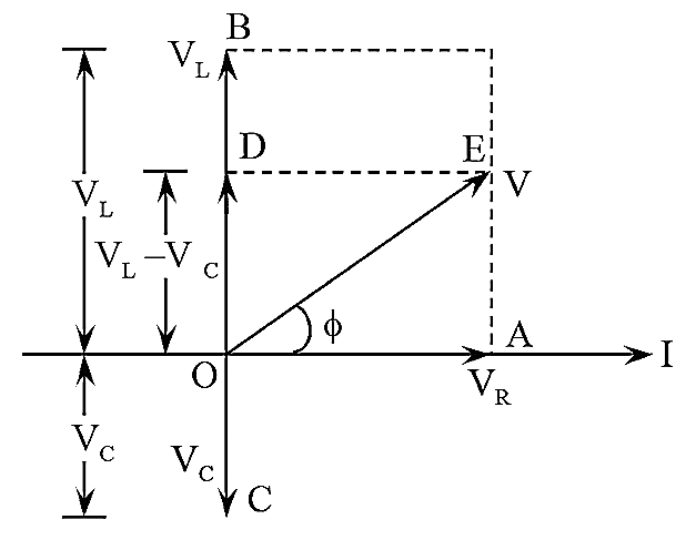
Phasor diagram corresponding to an LCR circuit

(Source : https://electricalworkbook.com/rlc-series-circuit/)

This diagram visualizes the information encapsulated by phasor notation.

At resonance in series LCR circuit, the current amplitude must be maximum. For fixed values V, R, L, C, the RHS of the expression is only affected by ω. And to maximize the fraction on the RHS (which is equal to the I^2), the denominator must be minimized.

This requires the frequency to take the unique value of : ω= 1/sqrt(LC)